Results
Based on the research of overall trends of tropical forest changes, we can see clearly from figure 5. Before the middle of 1980s, the area of each forest ecosystem decreased. Combining the human factors, a large number of tropical forests were replaced to cattle-ranching during these years, especially tropical dry forests. Thus I called this process deforestation stage. After that, however, the government of Costa Rica who had realized the degraded situation was serious took a series of policies to prevent from continuous degradation and to encourage forest restoration. Moreover, because of the beef industry collapse, the areas of forests increased dramatically, almost rising up to, even exceeding the original state. This process was called restoration stage.
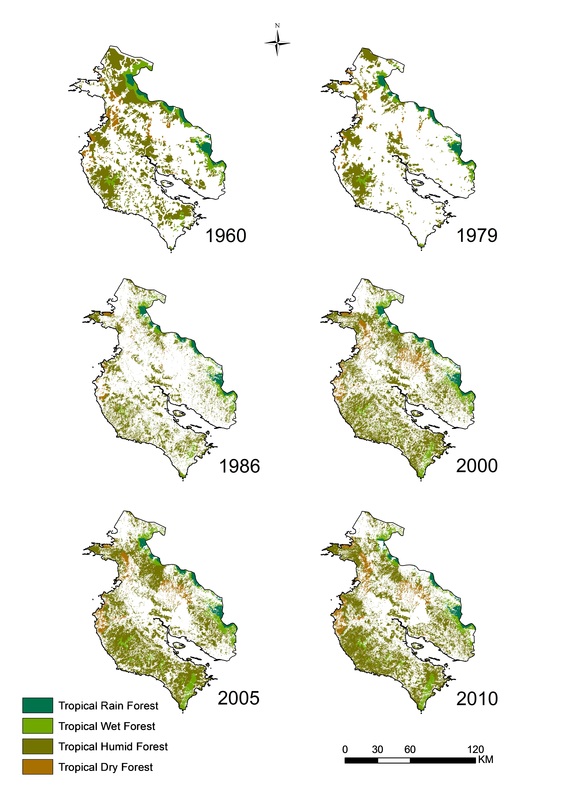
Figure 4. The Changes of Forests from 1960 to 2010
|
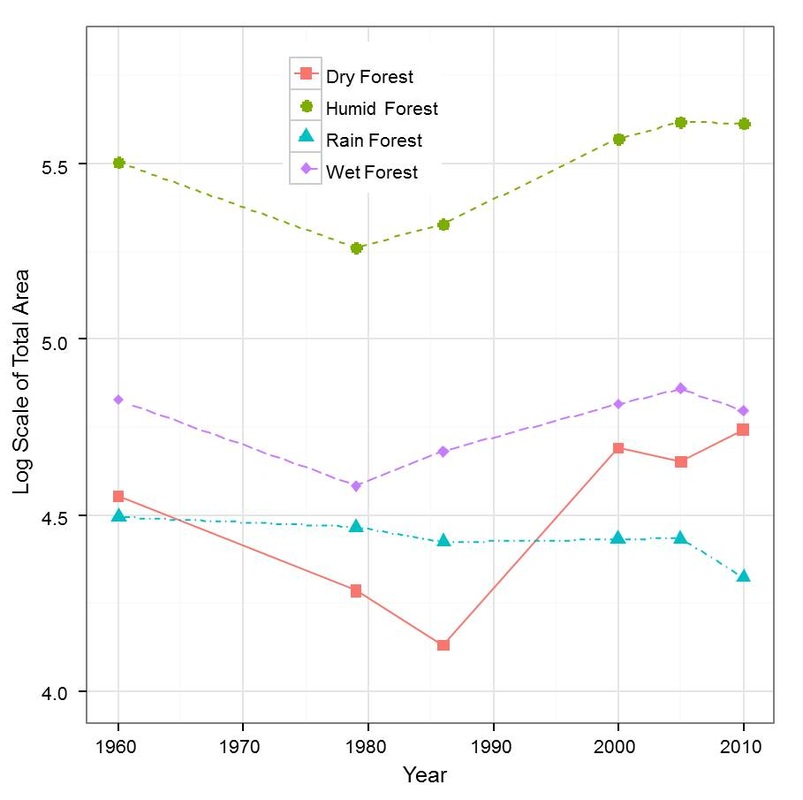
Figure 5. The Line Chart of Forest Changes
|
From the graphs of patches analysis, some conclusions could be found
(see figure 6).
The first one was patch area index (a). In the deforestation stage, patch areas
decreased significantly whereas it increased smoothly after that except rain
forest. The second one was shape index (b). This index did not vary
drastically, just some reasonable fluctuations. The next one was contiguity
index (c). For dry and rain forest, this index decreased in the deforestation
stage and kept stable after this period, but for the other forest, it increased
slightly in the restoration stage. The following was core area index (d). This
index decreased during degradation, but in the restoration stage, it did not
increase. The last one was Euclidean nearest neighbour index (e). This index
had the same trend as core area index. From the patches analysis, I got an interesting
result: although the area of forest rose up to the original state, forest
functions and spatial structures did not fully go up.


Figure 6. Patches Analysis
Thus I clustered these existing forest ecosystems according to these
landscape indices in the class level which represent forest function and
spatial structure. After dimensionality reduction (PCA), I got the first 5
principle components (PCs) which could explain 97.45% variance of total (see figure 7). Figure 8 showed the first 2 PCs and their loadings. I used these PCs as variables for
clustering analysis, and then 10 was used as a standard height. Based on the
functional and structural similarities of forests, forest ecosystems in
different years were separated into 4 groups (see figure 9). Each group had its own similar
forest function and spatial structure.

Figure 7. Scree Plot
|
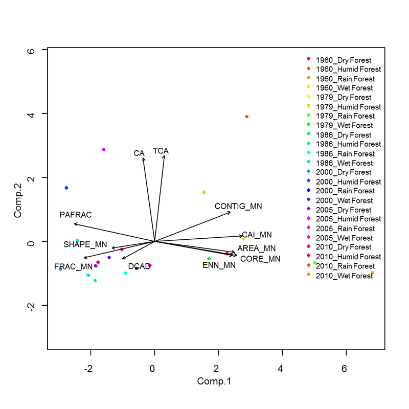
Figure 8. The First Two PCs and Their Loadings
|

Figure 9. Forests Clustering
|
